When a function is not continuous at a point within its domain, that point is called a discontinuity point. Based on the existence of limits, discontinuity points are generally divided into the following two categories and four types:

First-Kind Discontinuities

First-kind discontinuities refer to points where both left and right limits exist but the continuity condition is not satisfied, including removable discontinuities and jump discontinuities.

• Removable Discontinuity
  Condition:

  $$\lim_{x \to x_0^-} f(x) = \lim_{x \to x_0^+} f(x) = L \neq f(x_0) \quad\text{or } f(x_0)\text{ is undefined}$$

  Remedy:
  By redefining $f(x_0)=L$, the function becomes continuous at $x_0$.
  Typical Example: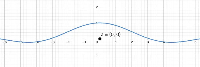

  $$f(x) = \begin{cases} \frac{\sin x}{x}, & x \neq 0 \\\\ 0, & x = 0 \end{cases}$$

  
  At $x=0$:

  $$\lim_{x \to 0} \frac{\sin x}{x} = 1 \quad\text{but } f(0) = 0$$

  Hence $x=0$ is a removable discontinuity.

• Jump Discontinuity
  Condition:

  $$\lim_{x \to x_0^-} f(x) = L_1 \quad\text{and}\quad \lim_{x \to x_0^+} f(x) = L_2 \quad\text{but } L_1 \neq L_2$$

  Irreparability:
  The jump amount $\Delta = \lvert L_2 - L_1\rvert$ cannot be eliminated by redefining $f(x_0)$.
  Piecewise Function Example: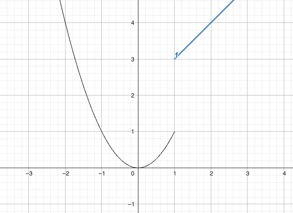

  $$f(x) = \begin{cases} x + 2, & x > 1 \\\\ x^2, & x \leq 1 \end{cases}$$

  
  At $x=1$:

  $$\lim_{x \to 1^-} x^2 = 1, \quad \lim_{x \to 1^+} (x+2) = 3$$

  The two-sided limits are not equal, so it is a jump discontinuity.

Second-Kind Discontinuities

Second-kind discontinuities are points where at least one side limit does not exist, or the limit “exists” but tends to infinity, including infinite discontinuities and oscillatory discontinuities.

• Infinite Discontinuity
  Characteristic:

  $$\lim_{x \to x_0} \lvert f(x)\rvert = +\infty$$

  The graph of the function exhibits a vertical asymptote near $x_0$.
  Typical Example: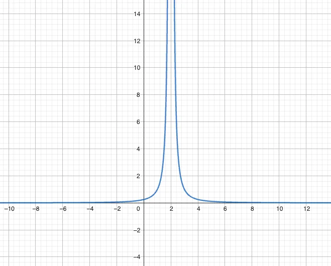

  $$f(x) = \frac{1}{(x-2)^2}$$

  
  At $x=2$:

  $$\lim_{x \to 2} \frac{1}{(x-2)^2} = +\infty$$

• Oscillatory Discontinuity
  Characteristic:
  The limit oscillates infinitely within a finite interval at a certain point, neither converging to a finite value nor diverging to infinity.
  Example Analysis: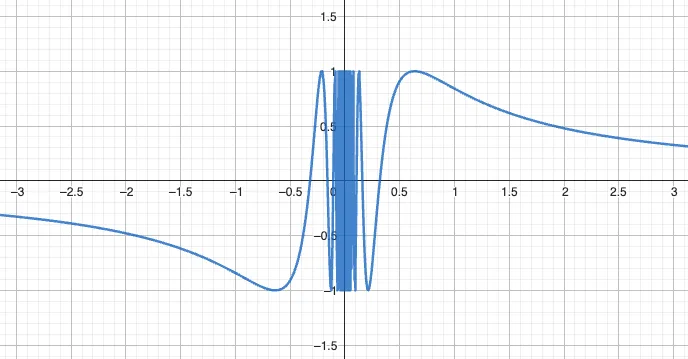

  $$f(x) = \sin\Bigl(\frac{1}{x}\Bigr)$$

  
  As $x \to 0$, $\frac{1}{x}$ increases without bound, causing $\sin\bigl(\frac{1}{x}\bigr)$ to oscillate infinitely in the interval $[-1,1]$, and both left and right limits do not exist. Hence $x=0$ is an oscillatory discontinuity.

Key Positions and Judgment Methods

When determining the discontinuity points of a function, it is usually necessary to focus on the following types of $x$ values, which are potential locations of discontinuities.

• Boundary Points of the Domain
  For example, the domain of $f(x)=\sqrt{x}$ is $[0,\infty)$. At $x=0$, the function is only defined on the right, so we need to check $\lim_{x \to 0^+} f(x)$. If the function has other smaller intervals, specific judgment of one-sided limits is required.

• Connection Points of Piecewise Functions
  If the function is given in piecewise form

  $$f(x) = \begin{cases} g(x), & x < a \\\\ h(x), & x \ge a \end{cases}$$

  then it is necessary to check at $x=a$: the relationship among $\lim_{x \to a^-} g(x)$, $\lim_{x \to a^+} h(x)$, and the function value $f(a)$.

• Denominator Zeros (Rational Functions)
  If $f(x) = \frac{P(x)}{Q(x)}$, first solve the equation $Q(x)=0$. For a point $x_0$ with $Q(x_0)=0$, also check whether $P(x_0)=0$.

  • If $P(x_0)\neq 0$, it is usually an infinite discontinuity.
  • If $P(x_0)=0$, simplify the fraction and then judge. For example, $$f(x)=\frac{x^2-1}{x-1},$$ at $x=1$ simplifies to $f(x)=x+1$ (for $x \neq 1$), indicating a removable discontinuity.

• Special Function Structure Points

Function Type	$x$ Values to Check	Typical Discontinuity Type
Logarithmic	$\ln[g(x)]$ where $g(x)\leq 0$	Second-kind discontinuity
Tangent	$\tan[g(x)]$ where $g(x)=\frac{\pi}{2}+k\pi$	Infinite discontinuity
Absolute Value	$\lvert x-a\rvert$ at $x=a$	Usually continuous (change in differentiability)

• Oscillatory Limit Points
  Functions containing $\sin\bigl(\tfrac{1}{x}\bigr)$, $\cos\bigl(\tfrac{1}{x}\bigr)$ and similar “high-frequency” oscillatory structures often exhibit infinite oscillation at certain points (commonly at $x=0$), requiring special attention.

• Connection Points of Composite Functions
  If the outer function imposes additional restrictions on the input, it is necessary to determine the range where the inner expression satisfies those restrictions. For example,
  $f(x)=\sqrt{\ln x}$ requires $\ln x \ge 0$ (i.e., $x \ge 1$), and we check the one-sided limit and function value at $x=1$.

Comprehensive Judgment Steps

After identifying candidate points to check, analyze them according to the following flowchart:

graph TD
    A[Compute left limit] --> B[Compute right limit]
    B --> C{Do limits exist?}
    C -->|Yes| D[First-kind analysis]
    C -->|No| E[Second-kind analysis]

For more detailed type determination, refer to the following diagram:

graph TD

    A[Point x_0 to check] --> B{Is f(x_0) defined?}

    B -->|Undefined| C[Compute left and right limits]
    B -->|Defined| C1[Compute left and right limits]

    C --> D{Do both left and right limits exist?}
    C1 --> D{Do both left and right limits exist?}

    D -->|No| E{Possible second-kind}
    E -->|If limit tends to ∞| F[Infinite discontinuity]
    E -->|If limit oscillates| G[Oscillatory discontinuity]

    D -->|Yes| H{Are left and right limits equal?}
    H -->|No| I[Jump discontinuity]

    H -->|Yes| J{Left limit = right limit = f(x_0)?}
    J -->|f(x_0) undefined or different| K[Removable discontinuity]
    J -->|Equal| L[Continuous point]

Example 1:
Analyze the discontinuity of

$$f(x)=\frac{e^{1/x}}{1+e^{1/x}}$$

at $x=0$:

• Since $f(0)$ is undefined, it is first judged as a discontinuity.
• Compute one-sided limits: $$\lim_{x \to 0^-} f(x) = 0, \quad \lim_{x \to 0^+} f(x) = 1.$$ The one-sided limits are not equal, so it is a jump discontinuity.

Example 2:
Determine the behavior of

$$f(x) = x \cos\Bigl(\tfrac{1}{x}\Bigr)$$

at $x=0$:

• The function is not explicitly defined at $x=0$, so it is initially considered a discontinuity.
• However, by the squeeze theorem:
  $-\lvert x\rvert \le x\cos\bigl(\tfrac{1}{x}\bigr) \le \lvert x\rvert$,
  we obtain
  $\lim_{x \to 0} x\cos\bigl(\tfrac{1}{x}\bigr) = 0$.
• By defining $f(0)=0$, the function becomes continuous at $x=0$. Hence the origin is a removable discontinuity.

Special Cases

• Connection Points of Piecewise Functions
  Compute the left and right limits separately, then compare with the function value at the connection point. If all three are equal, it is continuous; otherwise, it is a discontinuity.
  Example:

  $$f(x)= \begin{cases} e^x, & x<0 \\\\ x+1, & x\ge 0 \end{cases}$$

  At $x=0$:
  $\lim_{x \to 0^-} e^x = 1$, $\lim_{x \to 0^+} (x+1) = 1$, $f(0)=1$,
  all equal, so it is continuous.

• Existence of Derivative and Discontinuity
  If $f(x)$ is differentiable at $x_0$, then it must be continuous at $x_0$.
  However, a function may be non-differentiable at a point but still continuous, e.g., $f(x)=\lvert x\rvert$ is not differentiable at $x=0$ but remains continuous.