Uses function symbols with primes to denote derivatives. If y=f(x), then:
f′(x0)ory′
Features:
Directly associates with function names, making the correspondence between function and derivative clear
Higher-order derivatives are indicated by the number of primes: second derivative f′′(x), third derivative f′′′(x) Example: f(x)=x3 has derivative:
f′(x)=3x2f′′(x)=6x
Applicable scenarios:
Explicit function expressions (e.g., f(x)=sinx)
Theoretical proofs and formula derivations
Leibniz Notation
Uses differential symbols to represent derivatives. If y=f(x), then:
dxdyx=x0ordxdf(x)
Features:
Intuitively shows the derivative as the limit of a ratio of differentials
Higher-order derivatives are indicated by exponents: second derivative dx2d2y Chain rule example:
Let y=sin(u), u=x2, then:
dxdy=dudy⋅dxdu=cos(u)⋅2x=2xcos(x2)
Applicable scenarios:
Implicit functions (e.g., x2+y2=1)
Multivariable calculus and physical equations
Newton Notation
Uses dots above variables to denote time derivatives. If displacement is s(t), then:
s˙=dtds,s¨=dt2d2s
Features:
Concise notation, especially suitable for time derivatives
For derivatives beyond third order, multiple dots are used (e.g., s... for third derivative) Kinematics example:
Free fall motion s(t)=21gt2, then:
s˙=gt(velocity)s¨=g(acceleration)
Applicable scenarios:
Classical mechanics and dynamics problems
Systems of differential equations (e.g., vibration system x¨+ω2x=0)
Comparison and Selection Principles
Notation Type
Advantages
Limitations
Lagrange
Clear function relationship
Cumbersome notation for higher-order derivatives
Leibniz
Intuitive reflection of differential nature
Must note it is not a fraction
Newton
Efficient for time derivatives
Only applicable to single-variable time functions
For example, in the heat equation, mixing different notations is more efficient:
∂t∂T=α∇2T(Leibniz for spatial derivatives + Newton for time derivative)
Definition
The derivative of a function is defined as the limit of the ratio of the increment of the function to the increment of the independent variable as the increment of the independent variable approaches zero. Mathematically:
When the limit exists, the function y=f(x) is said to be differentiable at x0, and this limit is called the derivative of y=f(x) at point x0.
Essentially, the definition of derivative is a limit problem
From the definition, it can be seen that the derivative studies the trend of change speed through the ratio of the change in function value to the change in independent variable.
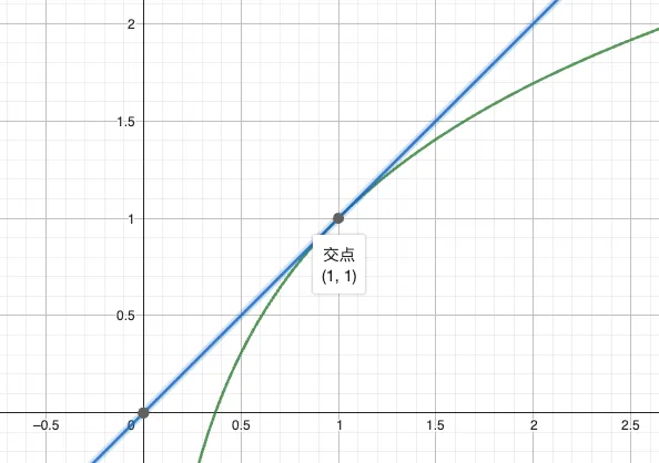
「From a graphical perspective, the derivative is the slope of the tangent line to the function y=f(x) at x=x0」
Verify that the function y=lnx+1 at x=1 has a tangent slope of 1, so the tangent is y−1=1⋅(x−1)
And here f′(x) at x=1 is indeed equal to 1
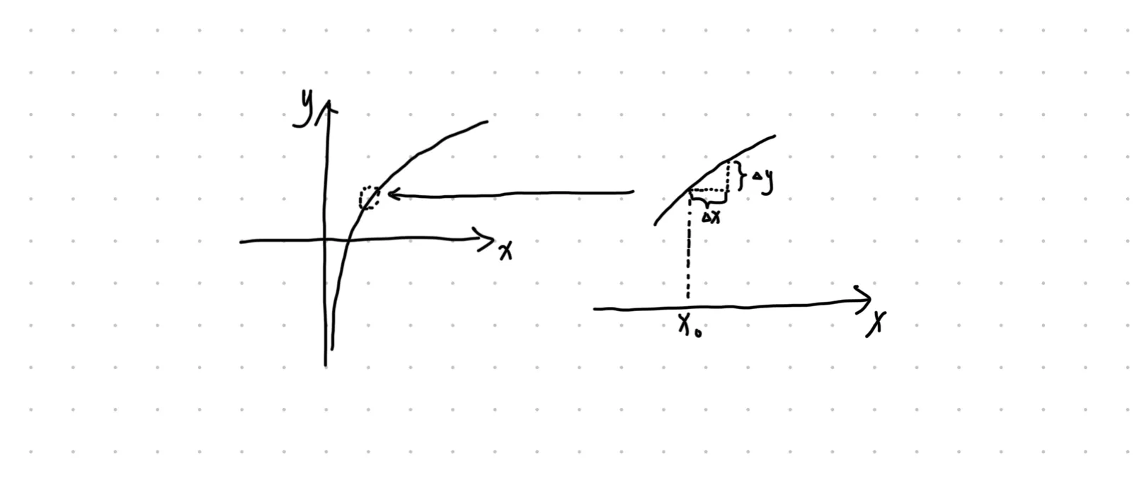
How to prove it more rigorously?
As can be seen in this illustration, when Δx→0, the points (x0,f(x0)) and (x0+Δx,f(x0+Δx)) approach a straight line. For this line, its slope is:
k=x0+Δx−x0f(x0+Δx)−f(x0)=Δxf(x0+Δx)−f(x0)
Does that look familiar?
Differentiation Rules
Basic Elementary Function Derivatives
Function Type
Derivative Formula
Constant function
(C)′=0
Power function
(xμ)′=μxμ−1
Exponential function
(ax)′=axlna
Natural exponential function
(ex)′=ex
Logarithmic function
(logax)′=xlna1
Natural logarithmic function
(lnx)′=x1
Sine function
(sinx)′=cosx
Cosine function
(cosx)′=−sinx
The derivative formulas for basic elementary functions can of course be derived using the definition of the derivative.
Operations
Addition and Subtraction Rule
(u±v)′=u′±v′
Product Rule
(uv)′=u′v+uv′
Quotient Rule
(vu)′=v2u′v−uv′
where u,v are basic elementary functions
Chain Rule
For composite functions, the derivative is obtained using the chain rule:
dxd[f(g(x))]=f′(g(x))⋅g′(x)
The chain rule states that the derivative of a composite function equals the derivative of the outer function with respect to the inner function multiplied by the derivative of the inner function. Intuitively, the rate of change of the rate of change equals the product of the individual rates of change.
Basic steps:
Identify the outer function and inner function in the composite function
Compute the derivative of the outer function, keeping the inner function unchanged
Compute the derivative of the inner function
Multiply the two derivatives to obtain the final result
where f+′(x0) and f−′(x0) are the right-hand and left-hand derivatives of f(x) at x=x0, collectively called one-sided derivatives.
Furthermore, for y=f(x), if at x=x0 the one-sided derivatives exist and are equal:
f+′(x0)=f−′(x0)
then f′(x) exists and equals the one-sided derivative value. (Sufficient and necessary condition)
Relationship between Differentiability and Continuity
From the above, it is easy to compare differentiability and continuity. The descriptions of these two properties are very similar, aren’t they?
Continuity
If a function f(x) is continuous at x=x0, then: f(x)=limx→x0+f(x)=limx→x0−f(x) Differentiability
If a function f(x) is differentiable at x=x0, then: f′(x)=f+′(x0)=f−′(x0)
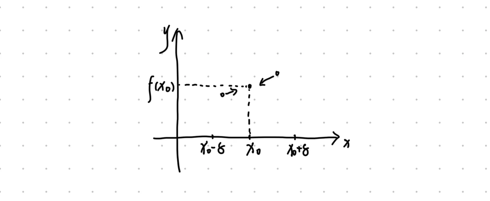
A function f(x) is continuous at x=x0 if and only if
∀ϵ>0,∃δ>0,such that when ∣x−x0∣<δ, we have ∣f(x)−f(x0)∣<ϵ.
That is, the result of applying the standard part function to all hyperreal numbers in a neighborhood centered at x0 is the real number f(x0).
A continuous interval consists of real numbers, but these real numbers are accompanied by infinitely close hyperreal numbers in the hyperreal model. Continuity in the hyperreal perspective is manifested as the stability of function values under infinitesimal perturbations, rather than a ‘seamless connection’ in space.
Clearly, the definition of continuity: f(x)=limx→x0+f(x)=limx→x0−f(x) essentially means that function f(x) is continuous at x0 if and only if for all hyperreal numbers x infinitely close to x0, f(x) is infinitely close to f(x0). Continuity is a local property, and the continuity of a function on an interval must be verified at each point individually. Hence we often see the description ‘the function is everywhere continuous on an interval’.
Alright, let’s continue with differentiability.
Definition of derivative:
f′(x0)=x→x0limx−x0f(x)−f(x0)
When the limit exists, the function is said to be differentiable. That is:
f′(x0)=∞
For the case f′(x0)=0, the numerator is a higher-order infinitesimal relative to the denominator. That is, f(x)−f(x0) approaches 0 faster than x−x0;
The expression for continuity at x=x0 is essentially f(x)−f(x0) approaches 0.
But differentiability requires a stronger condition than continuity: f(x)−f(x0) must approach 0 faster than x−x0.
For the case f′(x0)=a,a∈R, the numerator and denominator are infinitesimals of the same order.
Then differentiability also requires a stronger condition: f(x)−f(x0) and x−x0 must be infinitesimals of the same order.
Continuity and Differentiability Analysis of a Function and Its Absolute Value
Continuity
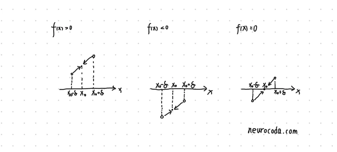
Assume there is a function f(x) that is continuous everywhere in its domain.
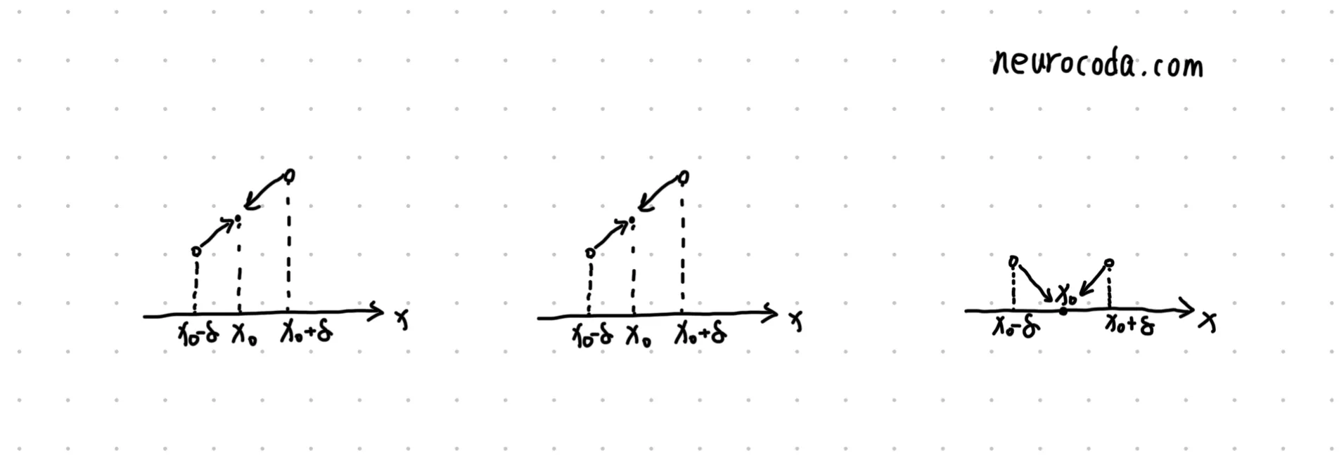
For f(x), according to the range of its values, it can be summarized into three possible cases as shown in the figure below:
For ∣f(x)∣, the corresponding cases are:
Clearly, if f(x) is continuous at a point, then ∣f(x)∣ is also continuous at that point. (After taking absolute value, hyperreal numbers in the neighborhood still approach that real point.)
So if ∣f(x)∣ is continuous at a point, can we prove that f(x) is also continuous at that point?
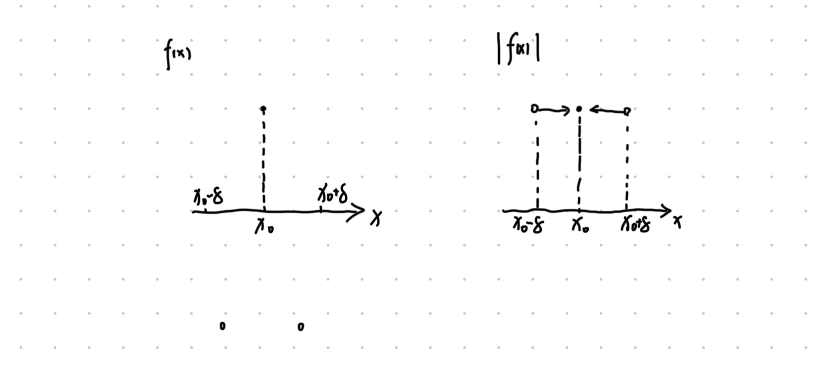
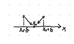
For f(x), according to the range of its values, it can be summarized into three possible cases as shown in the figure below:
For ∣f(x)∣, the corresponding cases are:
Regarding differentiability, as we just mentioned, differentiability requires a stronger condition than continuity, namely f(x)−f(x0) must approach 0 faster than x−x0.
This case satisfies continuity but does not satisfy f′(x)=f+′(x0)=f−′(x0).
Conclusion:
⎩⎨⎧f(x0) differentiablef(x0)=0⇒∣f(x0)∣ differentiable⎩⎨⎧f(x0) differentiablef(x0)=0f′(x0)=0⇒∣f(x0)∣ not differentiable
When f(x0)=0 and f′(x0)=0, the graph coincides with the x-axis, ∣f′(x0)∣=0.
The necessity has been described in the proof of continuity above and will not be repeated.
It can be summarized as:
f(x0) differentiable ⇔∣f(x0)∣ differentiable
Parity Relationship between Derivative and Original Function
First, give the conclusion:
⎩⎨⎧If f(x) is a differentiable even function, then f′(x) is an odd functionIf f(x) is a differentiable odd function, then f′(x) is an even function
Proof: If f(x) is a differentiable even function, then f′(x) is an odd function